The Equity Risk Premium (“ERP”) changes over time. Fluctuations in global economic and financial conditions warrant periodic reassessments of the selected ERP and accompanying risk-free rate.
Based upon market conditions as of December 31, 2018, Duff & Phelps increased its U.S. Equity Risk Premium recommendation from 5.0% to 5.5%. The 5.5% ERP guidance is to be used in conjunction with a normalized risk-free rate of 3.5% when developing discount rates as of December 31, 2018 and thereafter, until further guidance is issued. In summary:
- Equity Risk Premium: Increased from 5.0% to 5.5%
- Risk-Free Rate: Reaffirmed at 3.5% (normalized)
- Base U.S. Cost of Equity Capital: 9.0% (5.5% + 3.5%)
The Duff & Phelps recommended U.S. ERP as of December 31, 2018 was developed in relation to (and should be used in conjunction with) a 3.5% “normalized” risk-free rate. Some valuation professionals may prefer to use a spot (current market) risk-free rate, but the end result is that the base cost of equity capital should be approximately the same. Therefore, were one to use the spot yield-to-maturity on 20-year U.S. Treasuries as of December 31, 2018 (instead of a normalized 3.5%) one would have to increase the ERP assumption accordingly.
Background
The ERP is a key input used to calculate the cost of capital within the context of the Capital Asset Pricing Model (“CAPM”) and other models. Duff & Phelps regularly reviews fluctuations in global economic and financial market conditions that warrant a periodic reassessment of the ERP.1
Based on market conditions as of December 31, 2018, Duff & Phelps increased its recommended U.S. ERP from 5.0% to 5.5% when developing discount rates as of December 31, 2018 and thereafter, until there is evidence indicating equity risk in financial markets has materially changed and new guidance is issued.
Duff & Phelps last changed its U.S. ERP recommendation on September 5, 2017.2 On that date, our recommendation was decreased to 5.0% (from 5.5%) in response to evidence in early and mid-2017 that suggested a subdued level of risk in financial markets. Back then, strong earnings growth, still-accommodative monetary policies, and benign global macroeconomic trends buoyed U.S. stocks. Corporate earnings had surpassed expectations, fueling hopes for even higher dividend payouts and stock buybacks. Investors’ perception of negligible levels of risk was manifested through record-low levels of equity volatility and a sharp narrowing of corporate credit spreads.
The optimism in equity markets persisted into late 2017 and early 2018, after the passage into law of the largest U.S. corporate tax reform in over 30 years.3 The Tax Cuts and Jobs Act enacted on December 22, 2017 cut both personal income tax rates (temporarily through 2025) and the statutory corporate tax rate from 35% to 21% (permanently), among many other provisions. While not all industries were anticipated to be net beneficiaries from the U.S. tax reform, investors appeared to be expecting (on average) a substantial increase in after-tax corporate earnings, which spurred further stock market records. The combination of these upbeat economic and financial market conditions led Duff & Phelps to reaffirm its U.S. ERP recommendation of 5.0% as of December 31, 2017, to be used in conjunction with a normalized risk-free rate of 3.5%.4
February 2018 saw a spike in volatility, partly fed by concerns that a rise in inflation could lead to an acceleration in interest rate hikes. However, this proved to be temporary, with U.S. equity markets quickly bouncing back and reaching new record highs in September 2018.
From October through December 2018, the picture that emerged was very different: U.S. stock prices suffered significant losses, with an accompanying surge in equity volatility and a widening of corporate credit spreads. Broad U.S. stock market indices ended 2018 with negative total returns. This was the worst negative performance since 2008 at the height of the global financial crisis. The deterioration in economic indicators and financial market conditions led us to revisit our U.S. ERP recommendation.
Overview of the Duff & Phelps’ ERP Methodology
A Two-Dimensional Process
There is no single universally accepted methodology for estimating the ERP; consequently, there is wide diversity in practice among academics and financial advisors regarding ERP estimates. For this reason, Duff & Phelps employs a two-dimensional process that considers a broad range of economic information and multiple ERP estimation methodologies to arrive at its recommendation.
First, a reasonable range of normal or unconditional ERP is established. Second, based on current economic conditions, we estimate where in the range the true ERP likely lies (top, bottom, or middle).
Long-term research indicates that the ERP is cyclical.5 We use the term normal, or unconditional ERP to mean the long-term average ERP without regard to current market conditions. This concept differs from the conditional ERP, which reflects current economic conditions.6 The “unconditional” ERP range versus a “conditional” ERP is further distinguished as follows:
“What is the range?”
Unconditional ERP Range – The objective is to establish a reasonable range for a normal or unconditional ERP that can be expected over an entire business cycle. Based on an analysis of academic and financial literature and various empirical studies, we have concluded that a reasonable long-term estimate of the normal or unconditional ERP for the U.S. is in the range of 3.5% to 6.0%.7
“Where are we in the range?”
Conditional ERP – The objective is to determine where within the unconditional ERP range the conditional ERP should be, based on current economic conditions. Research has shown that ERP fluctuates during the business cycle. When the economy is near (or in) a recession, the conditional ERP is at the higher end of the normal, or unconditional ERP range. As the economy improves, the conditional ERP moves back toward the middle of the range and at the peak of an economic expansion, the conditional ERP approaches the lower end of the range.
Basis for Estimating the U.S. Equity Risk Premium as of December 31, 2018
Conditional Equity Risk Premium
In estimating the conditional ERP, valuation analysts cannot simply use the long-term historical ERP without further analysis. There is ample academic evidence that equity risk premia are not constant over time. Professor John Cochrane (senior fellow at the Hoover Institution at Stanford University) has summarized the changes in our knowledge of estimating rates of return for equity over the last 40 years, while emphasizing the need to adjust our valuation procedures and methodologies accordingly:8
“Discount rates vary a lot more than we thought. Most of the puzzles and anomalies that we face amount to discount-rate variation we do not understand. Our theoretical controversies are about how discount rates are formed. We need to recognize and incorporate discount-rate variation in applied procedures.”
Duff & Phelps goes beyond historical measures of ERP by examining approaches that are sensitive to the current economic and financial market conditions. In Exhibit 1, we list the primary factors considered when arriving at the Duff & Phelps recommended U.S. ERP: we document the evolution of these factors from December 31, 2017 through December 31, 2018, along with the corresponding relative impact on ERP indications.
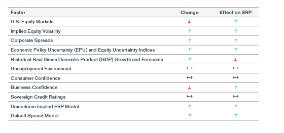
Exhibit 1: Factors Considered in the U.S. ERP Recommendation:
Relative Change from December 2017 to December 2018
Academic research shows that the Equity Risk Premium varies across business cycles. History alone may not capture risks faced by investors in the current environment.
Current Economic Conditions
Macroeconomic conditions provide the foundation for financial market performance, with economic growth influencing the level of interest rates, inflation, corporate earnings, and other factors that impact financial asset returns.
Global economic prospects improved markedly in late 2016 and during 2017. According to the International Monetary Fund (IMF), 2017 saw the broadest synchronized global growth upsurge since 2010.9 However, the geographic contribution to global growth was notably different in 2018, with the U.S. leading the pack, while other regions started seeing varying degrees of economic slowdown.
United States
Almost 10 years have elapsed since the U.S. economy began its recovery from the global financial crisis of 2008 (the “Financial Crisis”). The 2008–2009 U.S. recession was declared officially over in June 2009 and was of greater duration than those of 1973–1975 and 1981– 1982. The current business cycle expansion is now the second longest in U.S. history.10 However, the recent recovery has fallen short of the rebound observed in other post-World War II recessions. Real GDP growth in the year following the recessions of 1957–58, 1973– 75, and 1981–82 was on average 5.6%. In contrast, real GDP expanded by 2.6% during 2010 and by an average of 2.2% over the 2010–2017 period. Most economists believe that the long-term U.S. real GDP growth potential is now below the long-term historical trend of around 3.0%. (see Exhibit 2).11
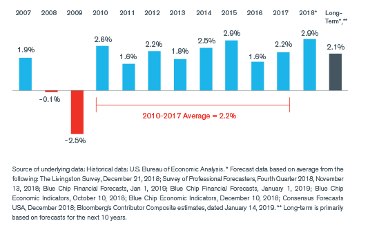
Exhibit 2: U.S. Real GDP Growth: 2007–2018 and Long-Term Forecasts at Year-end 2018 (approx.)
However, a spending boost fueled by individual and corporate tax cuts introduced in late 2017 by the Tax Cuts and Jobs Act, combined with a strong employment situation, restored optimism for 2018. As illustrated in Exhibit 2, U.S. real GDP is forecasted to have grown by a robust 2.9% in 2018, well above its projected long-term average (2.1%). Nevertheless, consensus among economists and professional forecasters point to a deceleration in economic activity in 2019 and beyond, as the effect of the fiscal stimulus gradually fades. Moreover, as discussed in more detail in the next section, a projected slowdown in global economic growth has the potential for negative spillover effects into the U.S. economy, a risk that worried investors in the fourth quarter of 2018.
The labor market had its best year in decades in 2018. The annual unemployment rate averaged 3.9%, the lowest level since 1969. During the second half of the year, the monthly unemployment rate oscillated between 3.7% and 3.9%, the former being the lowest monthly rate since 1969 while the latter had been last observed back in 2000 during the dot-com bubble.12
The economic theory underpinning the “Phillips Curve” suggests that a tight labor market and rapid economic growth can create upward pressure on wages and prices, leading to higher inflation.
Economic theory would suggest that a tight labor market and rapid economic growth would create upward pressure on wages and prices, ultimately leading to an increase in inflation. This relationship is often dubbed the “Phillips curve”.13 However, a significant increase in inflation has yet to be observed in the current U.S. economic recovery, which may imply that either the theory underlying the Phillips curve no longer holds, or that there is still some slack (i.e., unused capacity) in the U.S. economy not fully captured by the traditional unemployment rate measure (among other possible explanations).14,15
The Federal Reserve’s (“Fed”) preferred measures of inflation – the trailing 12-month personal consumption expenditures price index (PCE) and the core PCE (which excludes food and energy prices) – have remained below the U.S. central bank’s target rate of 2.0% until relatively recently. The first half of 2018 saw readings consistently near or exceeding 2.0%, which together with a strong labor market and robust real GDP growth, provided the Fed some comfort to continue to raise the target range of its benchmark short-term interest rate (the federal funds rate). However, by December 2018, the trailing 12-month PCE dipped again to 1.8%, while the core PCE ended the year at 2.0%. January 2019 saw further declines in both of these inflation measures.16 The trailing 12-month headline Consumer Price Index (CPI) and the core CPI (i.e., excluding food and energy) ended the year 2018 on a similar note. The headline CPI rose by 1.9% and the core CPI rose by 2.2% at the end of 2018, on a trailing 12-month basis.17
As discussed later in this document, the Fed’s monetary policy decisions during 2018 were a contributor to a tightening in financial market conditions and an increase in risk aversion in the last quarter of the year.
Global Economic Conditions
At the beginning of 2018, the expectations were for global economic growth to continue at similar levels to 2017. However, during the year, the rise of trade tensions – particularly between the U.S. and China – and the softening of the economic situation in China and Europe began to create uncertainty among companies and investors. Throughout the year, economic forecasts were progressively downgraded by major institutions and market participants.
For instance, in the March and May 2018 updates to its economic outlook the Organization for Economic Co-operation and Development (OECD) reported that global economic expansion was strengthening.18,19 By September, however, the OECD warned that global growth was hitting a plateau, and that risks from trade restrictions and tighter financial conditions had started to materialize in some countries.20 By November, the OECD concluded that, while strong, global GDP growth had already peaked, and that the 2019 growth forecasts had been lowered for most of the world’s major economies.21 Based on data observed in late 2018, the OECD became even more negative about the economic outlook, having revised its growth projections downward for most of the G-20 economies.22,23
Similarly, the IMF began 2018 on an optimistic note, but as the year progressed its global economic projections became bleaker. In April 2018, the IMF was still quite upbeat, citing supportive financial conditions as the reason to upgrade its 2018 and 2019 global growth rates to a level even higher than 2017. Additionally, the IMF stated that growth that strong and broad-based had not been seen since 2010, when the initial rebound from the Financial Crisis was observed.24
In July 2018, the IMF maintained its 2018 and 2019 projected global growth rates, but warned that the economic expansion was becoming less even, and that risks to the outlook were rising.25 The IMF conjectured that the rate of expansion had peaked in some major economies and growth had become less synchronized. In October 2018, shortly after the tenth anniversary of the Lehman Brothers collapse, the IMF portrayed a more unbalanced outlook.26 While growth in the U.S. remained remarkably robust, near-term prospects for the Eurozone, the United Kingdom, and China had deteriorated. Threats of retaliatory trade policies by the U.S., possible failure of Brexit negotiations, and tightening financial conditions for emerging markets, as these economies tried to adjust to the Fed’s progressive rate hikes, were cited as factors adding to the uncertainty.
After analyzing economic and financial market conditions prevailing in late 2018, the IMF released reports in early 2019 that showed a worsening trend in global economic conditions.27
The World Bank summarized the situation succinctly in its January 2019 global economic outlook: 28
“The outlook for the global economy has darkened. Global financing conditions have tightened, industrial production has moderated, trade tensions have intensified, and some large emerging market and developing economies have experienced significant financial market stress. Faced with these headwinds, the recovery in emerging market and developing economies has lost momentum. Downside risks have become more acute and include the possibility of disorderly financial market movements and an escalation of trade disputes.”
Quantitative Easing
Thus far, the global economic recovery has been supported by unprecedented monetary policies introduced after the Financial Crisis began. Since the onset of the crisis, the Fed and other major central banks – including the European Central Bank (“ECB”), the Bank of England (“BOE”), and the Bank of Japan (“BOJ”) – have (i) lowered their benchmark interest rates near or below 0.0% (zero); and (ii) implemented several rounds of unconventional quantitative easing (“QE”) measures.
The resulting sizable increases in these central banks’ balance sheets, along with various flight-to-quality episodes, have continued to exert a downward pressure on global long-term interest rates (see Exhibit 3).29
“The outlook for the global economy has darkened. (…) Downside risks have become more acute and include the possibility of disorderly financial market movements (…).”
Source: World Bank
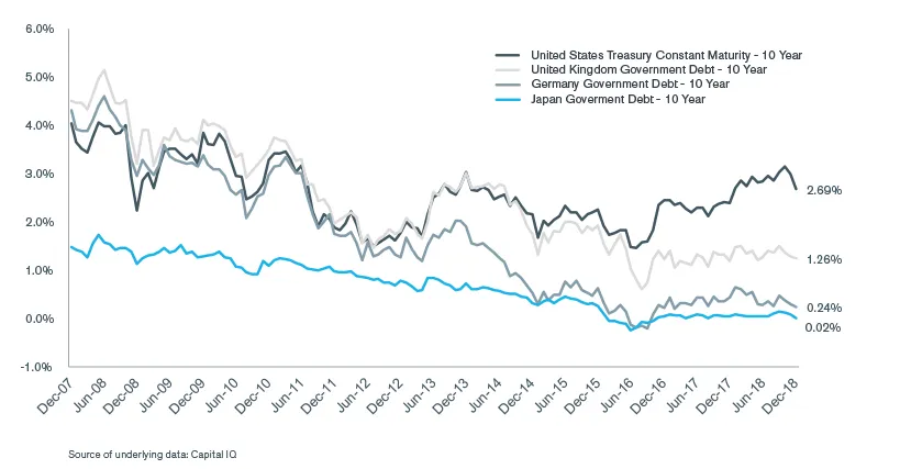
Exhibit 3: Yields on 10-year Government Bonds Issued by the U.S., U.K., Germany, and Japan, December 2007–December 2018
In the United States, the Fed kept a zero-interest-rate policy (dubbed “ZIRP” in the financial press) for seven years, from December 2008 until December 2015. In addition, the Fed purchased large quantities of long-term U.S. government securities, agency debt, and mortgage-backed securities (“MBS”). The Fed took both these actions with the objective of reducing long-term yields and boosting economic activity. These QE measures quickly expanded the Fed’s balance sheet from approximately $900 billion in early September 2008 to $4.5 trillion by September 2014.30
Various academic studies have suggested that the Fed’s QE policies significantly depressed the yields of long-term U.S. Treasury securities (thereby compressing the term premium). For example, in a recently released academic study (March 2018), the authors estimated that the cumulative effect of the Fed’s QE programs resulted in a reduction in the 10-year U.S. Treasury yield term premium of about 100 basis points (“b.p.”).31 For practical purposes, this is what this estimate would translate into: in absence of QE actions by the Fed, the 10-year yield of 2.69% as of December 31, 2018 would have potentially been around 3.69% instead. The authors also constructed a 90% confidence interval around their model estimates and indicated that the effect on the term premium could have been as small as 56 b.p. or as large as 140 b.p.32
Quantitative Tightening In December 2015, after a nearly 10-year period without interest rate hikes, the Fed finally embarked on a path of monetary policy normalization.33 As shown in Exhibit 4, the process started slowly, with the Fed raising the target range for the federal funds rate by 25 b.p. in December 2015 and again in December 2016. The pace accelerated in 2017, with three 25 b.p. rate increases during the year. Robust real economic growth, a strong job market, and inflation readings closer to its 2.0% target reinforced the case for the Fed to keep increasing interest rates in 2018. By the end of December 2018, the target range for the Fed’s benchmark rate had reached 2.25% to 2.50%, which was still relatively low by historical standards, but no longer considered unusual.
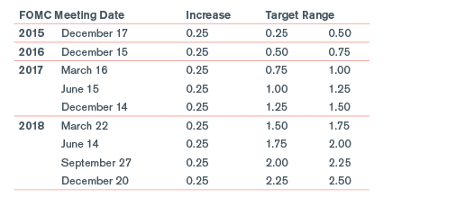
Exhibit 4: Federal Open Market Committee (FOMC) Interest Rate Hikes Since 2008 to Target Federal Funds Rate (%) 34
The impact of QE on interest rates is expected to diminish over time, as the Fed unwinds its portfolio of U.S. Treasuries, MBS, and agency debt. In its June 2017 meeting, the Fed revealed some details of its strategy to reduce its $4.5 trillion balance sheet. This gradual unwinding process, known as “quantitative tightening” (or “QT”) began in October 2017.
Exhibit 5 shows the schedule of securities held by the Fed that were allowed to expire (i.e., mature) each month under that new plan. In other words, the maximum monthly amount allowed to be removed from the Fed’s balance sheet. Under the plan, the Fed established two separate monthly caps: one for expiring U.S. Treasuries, and another for expiring MBS and agency debt. To the extent that the principal (in dollar amount) of the maturing securities (U.S. Treasuries + MBS + agency debt) is greater than the monthly cap, the excess is reinvested by the Fed. In contrast, if the principal of the maturing securities is less than the monthly cap, the Fed’s balance sheet goes down by the (lower) expired principal amounts.
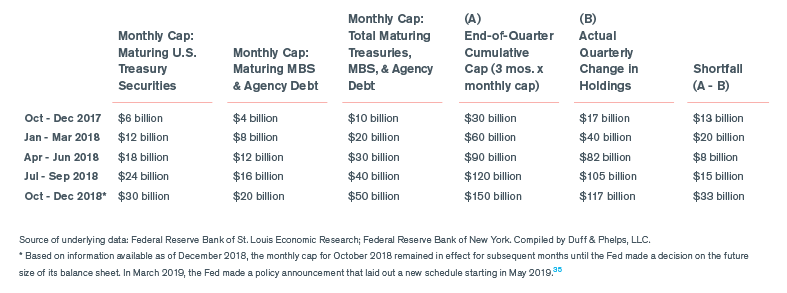
Exhibit 5: Monthly Caps and Actual Quarterly Reduction in Federal Reserve’s Security Holdings at December 2018
For example, during the calendar quarter of October through December 2017 (see the top row of Exhibit 5), the monthly cap of maturing U.S. Treasury securities was $6 billion, while the combined cap of MBS and agency debt was $4 billion, for an aggregate amount of $10 billion per month, or a $30 billion cap (3 months x $10 billion) for the whole quarter. However, the actual amount of U.S. Treasury securities, MBS, and agency debt that matured during the quarter was only $17 billion ($13 billion short of the maximum $30 billion cap for the quarter), and so the Fed’s balance of these securities declined $17 billion.
At the end of 2018 the size of the Fed’s balance sheet had declined to $4.1 trillion. Based on the plan outlined in Exhibit 5 and the pattern of balance sheet reductions seen thus far, it would not be unreasonable to conclude that the impact of QT would create only gradual (and arguably muted) upward pressure on interest rates.
James Bullard, President of the Federal Reserve Bank of St. Louis, stated as much in remarks delivered on February 22, 2019 at the 2019 U.S. Monetary Policy Forum in New York:36
“To summarize my argument, the financial and macroeconomic impact of the FOMC’s balance sheet policy may well be asymmetric. That is, the size of the balance sheet may have mattered while it was increasing but not while it has been decreasing. With the policy rate near zero, the effects of QE may have been substantial due to signaling effects. Now, with the policy rate well above zero, any signaling effects from balance sheet changes have dissipated. This means that balance sheet shrinkage, or QT, does not have equal and opposite effects from QE. Indeed, one may view the effects of unwinding the balance sheet as relatively minor.”
Despite the upbeat tone by the Fed in supporting interest rate hikes and the normalization of its balance sheet, investors became concerned that further rate rises would choke economic growth and corporate profits, especially given the strong signs of a global economic slowdown. On November 28, 2018, Fed Chairman Jerome Powell delivered a speech in which he discussed the outlook for the economy and the Fed’s monetary policy. His stance was that interest rates were still at historical lows and that they remained below the level that was considered neutral for the economy. He defined “neutral” as the level of interest rates that neither speeds up nor slows down the growth in the economy.37 Markets translated his comments as a clear indication that the Fed was determined to keep increasing rates further into 2019. Investors feared that such an interest rate path could potentially lead to a U.S. economic recession.
In Exhibit 6, we show how the 20-year U.S. Treasury yield – a typical proxy for the risk-free rate in U.S. dollars – and its 10-year trailing moving average have evolved from December 2007 through December 2018. From the beginning of the year until September 2018, with the economy growing at a fast pace, long-term government yields kept rising in tandem with the Fed’s increase in its benchmark short-term rate. During this period, the 20-year yield surpassed its trailing moving average for the first time in September 2018, a sign that perhaps long-term interest rates were finally moving upwards to historical levels. However, shortly after equity markets peaked, the 20-year yield started to decline again, ending the year at 2.9%, below its 10-year moving average of approximately 3.1%. With the Fed’s continued rise of its benchmark rate and consequent upward pressure on short term rates, the spread between short and long- term rates started to compress. This flattening of the yield curve stoked renewed fears that it could potentially be a signal or precursor to a U.S. recession.
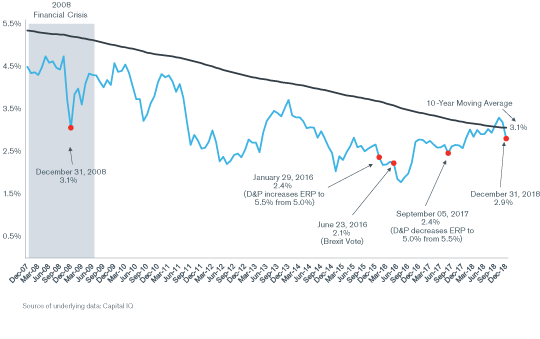
Exhibit 6: Spot and 10-Year Moving Average of Yields on 20-year U.S. Government, December 2007–December 2018
The speed of normalization of monetary policy in the U.S. and other advanced economies, mainly the Eurozone and Japan, was a major concern for markets because of the impact it has on currencies and interest rates. In June 2018, the ECB confirmed that the central bank would continue with the the same level of net monthly asset purchases until the end of September 2018. However, in that same meeting the ECB announced that it would cut in half the pace of net monthly asset purchases made between October to December 2018, at which point it would stop expanding its balance sheet.38 Similarly, in April 2018, Haruhiko Kuroda, the BOJ’s governor, mentioned that internal central bank discussions had begun regarding options for exiting the bank’s massive “Quantitative and Qualitative Monetary Easing (QQE) with Yield Curve Control” program. However, Mr. Kuroda told the Japanese parliament that it was too early to give any details about the plan. Furthermore, in July 2018 concerns that the BOJ might scale back its monetary policy shook global bond markets. The BOJ was forced to intervene multiple times to calm markets. Governor Kuroda indicated in a press conference that the BOJ would not be diverted from its stimulus program, even as other major central banks (including the Fed, the ECB and even the BOE) reversed their own QE programs.39
The IMF expressed concerns about the speed of normalization especially in the current environment and warned that these normalizations should consider the new realities on the ground. There are major concerns about the state of the economy in China – the second economy in the world – that could be aggravated by a prolonged trade tension with the U.S. On the European front, Brexit uncertainty, German economic slowdown, French street riots against proposed economic reforms, and the turmoil in Italian politics are other major events that could throw the regional European economy in serious danger and cause a slowdown in the overall global growth.40
“Monetary policy in advanced economies should continue to normalize carefully. The major central banks are keenly aware of the slowing momentum—and we expect they will calibrate their next steps in line with these developments. Macroprudential tools should be used where financial vulnerabilities are building up. Across all economies, measures to boost potential output growth and enhance inclusiveness are imperatives.”
Consumer and Business Confidence
A strong labor market and continued economic expansion helped consumers remain confident about the U.S. economy. As measured by the University of Michigan Consumer Sentiment Index, in December 2018 consumer confidence was slightly above the level observed at the end of 2017 and it was well above its long-term average.
However, the fear of a global economic slowdown and an increase in borrowing costs eroded businesses’ confidence in the future. The Business Confidence Index (BCI), published by the OECD, provides a survey-based indicator that compiles business leaders’ opinions in the industry sector and predicts turning points in economic activity. Index numbers above 100 suggest an increased confidence in near future business performance, whereas numbers below 100 indicate pessimism towards future performance. As illustrated in Exhibit 7, the BCI was trending upward all of 2017 and beginning of 2018. However, it peaked in September 2018 (about the same time that equity markets peaked) and started to head down towards the 100 level. This implied that as of December 2018, businesses were expecting some softness in the economy.
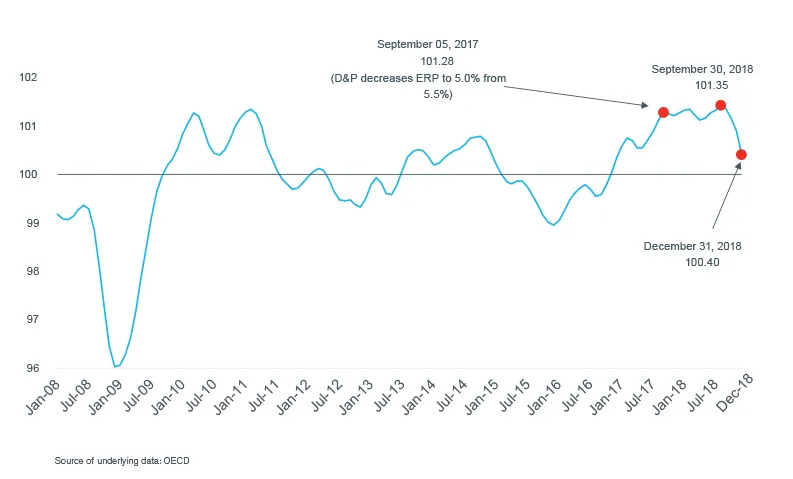
Exhibit 7: OECD Business Confidence Indicator (BCI) - United States, December 31, 2007–December 31, 2018
Current Financial Market Conditions
The last time Duff & Phelps changed its U.S. ERP recommendation was on September 5, 2017, (from 5.5% to 5.0%) and it was reaffirmed on December 31, 2017. Since then, aggregate risks in U.S. markets appear to have increased.
U.S. Equity Markets
2018 marked the tenth anniversary of the Financial Crisis and the longest bull market in history. By the end of the third quarter, equity markets registered their highest record yet. The NASDAQ Composite index set an all-time high of 8,109.69 on August 29, 2018, the S&P 500 index reached a record high on September 20 by closing at 2,930.75, and the Dow Jones Industrial Average closed at its highest level ever on October 3 at 26,828.39. With the beginning of the fourth quarter, the trend started to falter and market performance started to turn negative. The month of October saw the S&P 500 lose 6.94% of its index value (in price terms), whereas the Dow and Nasdaq lost 5.07% and 9.2% respectively.
While major market indices saw negative returns in the month of October, performance was even more dismal in December 2018. As a result, 2018 marked the worst annual performance for U.S. equity markets since the Financial Crisis. Overall, the Dow Jones Industrial Average declined 5.6% (in price terms), whereas the S&P 500 and the NASDAQ lost 6.2% and 3.9% of their respective index values.
As illustrated in Exhibit 8, the S&P 500 index gained 9.6% since December 31, 2017 until September 20, 2018, when it reached a record high. Shortly after the Fed’s meeting decision on September 26 to raise its benchmark interest rate by 25 b.p., while also showing no intent to slow its path towards normalization, markets reversed their ascent. Losses continued after the Fed’s December 19th meeting decision of yet another 25 b.p. hike. Between the record high achieved on September 20 and December 24, the lowest level for the index reached during 2018, the S&P 500 index declined by 19.8%. Some financial market commentators argued that U.S. major equity indices had reached a bear market.41

Exhibit 8: S&P 500 Index Performance, December 31, 2017–December 31, 2018
The rout in equity markets during the fourth quarter of 2018 was not confined to the United States. Most global equity markets were down during this period. Global investors were concerned by some of the same factors as those cited by U.S. investors, including trade tensions between the U.S. and its major partners (especially with China), a tightening in monetary policy by major central banks, faltering global economic growth – especially in China, Germany, and Japan – with its corresponding impact on corporate earnings growth, Brexit uncertainty, and political turmoil in Italy and other markets. The MSCI All Country World Index (ACWI), an index covering stocks across 23 developed markets and 24 emerging market countries, declined by 13.1% in the fourth quarter of 2018. Similarly, the MSCI EAFE, an index of stocks in 21 developed markets that excludes the U.S. and Canada, dropped by 12.9% over the same period.42
Implied Equity Volatility
Implied equity volatility, as measured by the Chicago Board Options Exchange (CBOE) “VIX” Index, has been termed a “fear index” as it can be a gauge of investor apprehension. Volatility in the U.S. equities market declined sharply in late 2016 and during 2017. The beginning of 2018 saw a spike in volatility that lasted two months; however strong corporate earnings and the high consumer confidence calmed investors’ fears and pushed markets higher. The volatility came back by the end of 2018, as investors appeared much more nervous about financial markets than earlier in the year. The average daily VIX during the last quarter of 2018 (21.1) was practically double the average VIX during all of 2017 (11.1). As shown in Exhibit 9, during 2018 the VIX Index peaked on December 24, 2018, the same day that the S&P 500 reached its lowest level for the year.
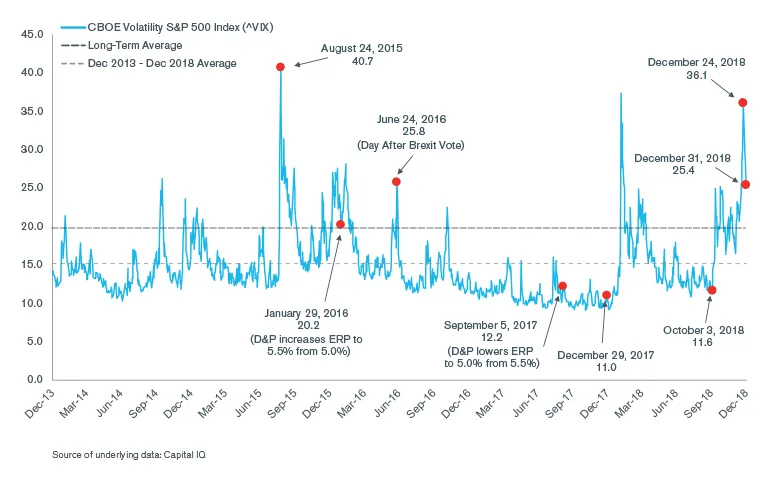
Exhibit 9: Chicago Board Options Exchange (CBOE) “VIX” Index, December 2013–December 2018
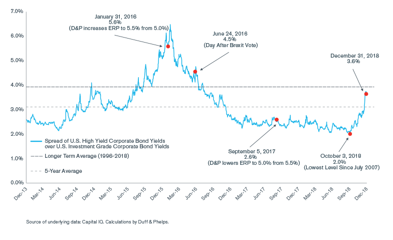
Exhibit 10: Spread of U.S. High-Yield Corporate Bond Yields over U.S. Investment Grade Corporate Bond Yields, December 2013–December 2018
Corporate Credit Spreads
Relative to December 2017, U.S. corporate credit spreads have widened substantially by year-end 2018 (see Exhibit 10). However, the surge in borrowing costs for non-investment grade (i.e., high-yield) corporate borrowers did not start until the fourth quarter of 2018. In fact, on October 3, 2018 (shortly after equity markets reached a new record high), the credit spread of U.S. high-yield over investment-grade corporate bonds reached its lowest level since July 2007, prior to the onset of the Financial Crisis.
Since the onset of the Financial Crisis, fixed income markets have been significant beneficiaries of the QE policies implemented by major central banks across the globe. Large asset purchases by central banks have created an environment of ultra-low interest rates, encouraging new corporate debt issuance on a global basis. In addition, QE programs in the Eurozone, United Kingdom, and Japan include investment-grade corporate debt securities, thereby decreasing borrowing costs for those corporations even further.
As mentioned earlier, a variety of factors, including Fed’s continued path towards monetary policy tightening, U.S. trade policy uncertainties (especially with China), signs of a global economic slowdown, and concerns about the outlook for corporate earnings all contributed to a deterioration in risk sentiment early in the fourth quarter of 2018. During this time, corporate bond spreads widened notably, particularly in December. In fact, in December 2018 the volume of high-yield bonds issued by nonfinancial firms dropped to zero, the first time that happened since 2008, according to data-provider Dealogic.43
Additional Indicators Supporting the ERP Change – Quantitative Models
In addition to the general economic factors and financial market conditions described above, Duff & Phelps monitors other indicators that may provide a more quantitative view of where we are within the range of reasonable long-term estimates for the U.S. ERP.
Duff & Phelps currently uses several models as corroborating evidence. We reviewed the following indicators at the end of December 2018:
- Damodaran Implied ERP Model – New York University Professor Aswath Damodaran calculates implied ERP estimates for the S&P 500 and publishes his estimates on his website. Prof. Damodaran estimates an implied ERP by first solving for the discount rate that equates the current S&P 500 index level with his estimates of cash distributions (dividends and stock buybacks) in future years. He then subtracts the current yield on 10-year U.S. government bonds to arrive at an implied ERP. Prof. Damodaran allows the user to select a variety of methods to project cash flow yields, as well as several expected growth rate choices for the terminal year in the valuation. Duff & Phelps converts Prof. Damodaran’s implied ERP estimates to an arithmetic average equivalent measured against the 20-year U.S. government bond yield, relying primarily on two measures of projected cash flows: (i) the trailing 12-month cash flow yield (dividends plus buybacks) of S&P 500 constituents; and (ii) the trailing 10-year average cash flow yield (dividends plus buybacks) of S&P 500 constituents.44
- Based on Prof. Damodaran’s estimates of the trailing 12-month cash flow yield, the implied ERP (converted into an arithmetic average equivalent) was approximately 7.20% at end of December 2018, when measured against an abnormally low 20-year U.S. government bond yield (2.87%).45 The equivalent normalized implied ERP estimate was 6.57% measured against a normalized 20-year U.S. government bond yield of 3.5%. This normalized implied ERP estimates represent an increase of 118 b.p., relative to the December 2017 estimate (5.38%). The normalized implied ERP indications were even higher in October and November 2018 (using the same methodology).
- Default Spread Model (DSM) – The Default Spread Model is based on the premise that the long-term average ERP (the unconditional ERP) is constant and deviations from that average over an economic cycle can be measured by reference to deviations from the long-term average of the default spread between corporate bonds rated in the Baa category by Moody’s versus those in the Aaa rating category. This model notably removes the risk-free rate itself as an input in the estimation of ERP.46 However, the ERP indication resulting from the DSM is still interpreted as an estimate of the relative return of stocks in excess of risk-free securities.
- At the end of December 2018, the conditional ERP calculated using the DSM model was 5.37%. This represents an increase of 44 b.p., relative to the 4.93% ERP indication at the end of December 2017. For perspective, March 2016 was the last time that the conditional ERP calculated using the DSM model was this high. As a reminder, this was also around the same time Duff & Phelps had increased its U.S. recommended ERP from 5.0% to 5.5%.47
Conclusion
Based on market conditions, prevailing at year-end 2018, we found sufficient evidence for increasing the Duff & Phelps U.S. ERP recommendation from 5.0% to 5.5%, for valuation dates as of December 31, 2018 and thereafter. We will maintain our recommendation to use a 5.5% U.S. ERP when developing discount rates until there is evidence indicating equity risk in financial markets has materially changed. We are continuing to closely monitor the economic outlook and financial market conditions. While financial markets may see a rebound from the depressed year-end levels, we will carefully evaluate whether the combined trends in the risk factors we regularly review warrant a change in our recommendation.
The current ERP recommendation was developed in conjunction with a “normalized” 20-year yield on U.S. government bonds as a proxy for the risk-free rate. Based on recent academic literature and market evidence of a secular decrease in real interest rates (a.k.a. the “rental” rate) and lower long-term real GDP growth estimates for the U.S. economy, we are reaffirming our concluded normalized risk-free rate of 3.5%, established as of November 15, 2016.48
The combination of the new U.S. recommended ERP (5.5%) and the reaffirmed normalized risk-free rate (3.5%) results in an implied U.S. “base” cost of equity capital estimate of 9.0% (5.5% + 3.5%).
Adjustments to the ERP or to the risk-free rate are, in principle, a response to the same underlying concerns and should result in broadly similar costs of capital. Adjusting the risk- free rate in conjunction with the ERP is only one of the alternatives available when estimating the cost of equity capital. Were one to use the spot yield-to-maturity of 2.9% on 20-year U.S. Treasuries as of December 31, 2018, one would have to increase the ERP assumption accordingly. One can determine the ERP against the spot 20-year yield as of December 31, 2018, inferred by Duff & Phelps’ recommended U.S. ERP (used in conjunction with the normalized risk-free rate), by using the following formula:

1. For a more detailed discussion of some of the studies and factors we evaluate, refer to Chapter 3 of the Duff & Phelps 2019 Valuation Handbook – U.S. Guide to Cost of Capital, available exclusively online through the Duff & Phelps Cost of Capital Navigator at dpcostofcapital.com.
2. Refer to the Duff & Phelps Client Alert issued on October 30, 2017, which was titled “Duff & Phelps’ U.S. Equity Risk Premium Recommendation Decreased from 5.5% to 5.0%, Effective September 5, 2017”. To obtain a free copy of this Client Alert and prior ones documenting the Duff & Phelps’ U.S. ERP recommendation over time, visit: www.duffandphelps.com/CostofCapital.
3. See, for example, Paletta, Damian and Stein, Jeff, “Sweeping tax overhaul clears Congress” The Washington Post, December 20, 2017. This article is accessible here.
4. For a more detailed discussion of this decision, refer to Chapter 3 of the Duff & Phelps 2018 Valuation Handbook – U.S. Guide to Cost of Capital, available exclusively online through the Duff & Phelps Cost of Capital Navigator at dpcostofcapital.com.
5. See for example John Cochrane’s “Discount Rates. American Finance Association Presidential Address” on January 6, 2011, where he presented research findings on the cyclicality of discount rates in general. His remarks were published as Cochrane, J. H. (2011), “Presidential Address: Discount Rates,” The Journal of Finance, 66: 1047–1108, available at https://onlinelibrary.wiley.com/doi/10.1111/j.1540-6261.2011.01671.x/full.
6. The “conditional” ERP is the ERP estimate published by Duff & Phelps as the “Duff & Phelps Recommended U.S. ERP”
7. See Shannon P. Pratt and Roger J. Grabowski, Cost of Capital: Applications and Examples, Fifth Edition, Chapter 8 “Equity Risk Premium”, and accompanying Appendices 8A and 8B, for a detailed discussion of the unconditional ERP. This discussion has been updated with more recent data in Chapter 3 of the Duff & Phelps 2019 Valuation Handbook – U.S. Guide to Cost of Capital, available exclusively online through the Duff & Phelps Cost of Capital Navigator at dpcostofcapital.com.
8. John C. Cochrane (2011), “Presidential Address: Discount Rates,” The Journal of Finance, 66: 1047–1108
http://onlinelibrary.wiley.com/doi/10.1111/j.1540-6261.2011.01671.x/full.
9. “World Economic Outlook Update, January 2018 – Brighter Prospects, Optimistic Markets, Challenges Ahead”, International Monetary Fund.
Accessible here: https://www.imf.org/en/Publications/WEO/Issues/2018/01/11/world-economic-outlook-update-january-2018.
10. “U.S. Business Cycle Expansions and Contractions”, National Bureau of Economic Research. https://www.nber.org/cycles.html.
11. Source of historical real GDP growth data: U.S. Bureau of Economic Analysis, http://www.bea.gov.
12. Source of historical monthly and annual unemployment rates: U.S. Bureau of Labor Statistics, Civilian Unemployment Rate, https://www.bls.gov/
13. The inverse relationship between inflation and unemployment is captured by the so-called “Phillips curve,” named after economist A. W. Phillips for his work in the 1950s. For a more detailed discussion on variations and extensions of the Phillips curve, as well as how well it captures the relationship between employment and inflation, see for example Peach, Richard, Robert Rich, and Anna Cororaton (2011), “How Does Slack Influence Inflation?”, Current Issues in Economics and Finance, Volume 17, Number 3, Federal Reserve Bank of New York. Available here: https://www.newyorkfed.org/medialibrary/media/research/current_issues/ci17-3.pdf.
14. St. Louis Federal Reserve bank president James Bullard explains in a presentation in 2018 ECB Forum on Central Banking that the empirical relationship between unemployment and inflation disappeared. Presentation can be accessed here: https://www.stlouisfed.org/~/media/files/pdfs/bullard/remarks/2019/bullard_usmpf_22_february_2019.pdf?la=en.
15. The official unemployment rate, labeled as U-3 by the U.S. Bureau of Labor Statistics, is comprised of total unemployed workers, as a percent of the civilian labor force. U-6, a broader definition of the unemployment rate, is computed using the following ratio: [Total Unemployed (U-3) + All Persons Marginally Attached to the Labor Force + Total Employed Part Time for Economic Reasons] / [Civilian Labor Force + All Persons Marginally Attached to the Labor Force]. The U-6 measure was 7.6% in December 2018. Source: https://www.bls.gov/.
16. U.S. Bureau of Economic Analysis, Personal Consumption Expenditures Price Index. Data can be found in the “Personal Income and Outlays” release, Table 11. Price
Indexes for Personal Consumption Expenditures: Percent Change From Month One Year Ago. For the latest release and access to previously published monthly estimates,
visit: https://www.bea.gov/data/personal-consumption-expenditures-price-index.
17. U.S. Bureau of Labor Statistics, CPI-All Urban Consumers (Current Series), available at: http://www.bls.gov. CPI inflation is based on the “All Items in U.S. City Average, All
Urban Consumers” series, whereas core CPI inflation is based on the “All Items less Food and Energy in U.S. City Average, All Urban Consumers” series.
18. Pereira, Álvaro, “Getting stronger, but tensions are rising,” oecdecoscope, March 13, 2018. Accessed here: https://oecdecoscope.blog/2018/03/13/getting-stronger-but-tensions-are-rising/.
19. Pereira, Álvaro, “Stronger Growth but Risks loom large,” oecdecoscope, May 30, 2018. Accessed here: https://oecdecoscope.blog/2018/05/30/stronger-growth-but-risks-loom-large/.
20. Boone, Laurence, “High uncertainty is weighing on global growth,” oecdecoscope, September 20, 2018.
Accessed here: https://oecdecoscope.blog/2018/09/20/high-uncertainty-is-weighing-on-global-growth/.
21. Boone, Laurence, “Editorial: Growth has peaked: Challenges in engineering a soft landing,” OECD Economic Outlook November 2018.
Accessed here: https://www.oecd.org/economy/outlook/growth-has-peaked-challenges-in-engineering-a-soft-landing.htm
22. Boone, Laurence, “Global growth is weakening: coordinating on fiscal and structural policies can revive euro area growth,” oecdecoscope, March 6, 2019. Accessed here: https://oecdecoscope.blog/2019/03/06/global-growth-is-weakening-coordinating-on-fiscal-and-structural-policies-can-revive-euro-area-growth/.
23. The G-20 is comprised of 19 countries plus the European Union (EU). The 19 countries are Argentina, Australia, Brazil, Canada, China, France, Germany, India, Indonesia, Italy, Japan, Mexico, Russia, Saudi Arabia, South Africa, South Korea, Turkey, United Kingdom, and United States. For more details visit: https://g20.org/en/
24. “World Economic Outlook, April 2018 – Cyclical Upswing, Structural Change”, International Monetary Fund. Accessible here: https://www.imf.org/en/Publications/WEO/Issues/2018/03/20/world-economic-outlook-april-2018.
25. “World Economic Outlook Update, July 2018 – Less Even Expansion, Rising Trade Tensions”, International Monetary Fund. Accessible here: https://www.imf.org/en/Publications/WEO/Issues/2018/07/02/world-economic-outlook-update-july-2018.
26. “World Economic Outlook, October 2018 – Challenges to Steady Growth”, International Monetary Fund.Accessible here: https://www.imf.org/en/Publications/WEO/Issues/2018/09/24/world-economic-outlook-october-2018.
27. “World Economic Outlook Update, January 2019 – A Weakening Global Expansion”, International Monetary Fund. Accessible here: https://www.imf.org/en/Publications/WEO/Issues/2019/01/11/weo-update-january-2019. In its April 2019 update, the IMF projected a slowdown in 2019 growth for 70% of the world economy. The downward revision reflected weaker projected growth for several major economies, including the Eurozone, Latin America, the United Kingdom, Canada, Australia, and even the United States “World Economic Outlook, April 2019 – Growth Slowdown, Precarious Recovery”, International Monetary Fund. Accessible here: https://www.imf.org/en/Publications/WEO/Issues/2019/03/28/world-economic-outlook-april-2019.
28. World Bank, “Global Economic Prospects: Darkening Skies”, January 2019, Washington, D.C. Available here: http://documents.worldbank.org/curated/en/307751546982400534/Global-Economic-Prospects-Darkening-Skies.
29. The ECB’s QE program includes purchases of euro-denominated investment-grade bonds issued by non-financial corporations. Besides commercial paper and corporate bonds, the Bank of Japan’s QE program includes significant purchases of equity securities through ETFs (exchange-traded funds) and Japan real estate investment trusts (J-REITs).
30. Source: Credit Easing, Federal Reserve Bank of Cleveland. Available here: https://www.clevelandfed.org/our-research/indicators-and-data/credit-easing.aspx
31. Ihrig, Jane; Klee, Elizabeth; Li, Canlin, Wei, Min and Kachovec, Joe. “Expectations about the Federal Reserve’s Balance Sheet and the Term Structure of Interest Rates.” International Journal of Central Banking, March 2018, 14(2), pp. 341-91. Accessible here: https://www.ijcb.org/journal/ijcb18q1a8.htm.
32. Some researchers have argued that Fed actions and announcements are not dominant determinants of the 10-year yield. In their opinion, any effect that the Fed actions might have on the long-term yield does not persist. Greenlaw, David, James D. Hamilton, Ethan Harris, and Kenneth D. West. “A Skeptical View of the Impact of the Fed’s Balance Sheet” (June 2018). NBER Working Paper No. w24687. Available at NBER: https://www.nber.org/papers/w24687.
33. The last time the Federal Open Market Committee’s (FOMC) had raised the target federal funds rate was in June 2006.
For a list of prior FOMC decisions and historical materials by year, visit https://www.federalreserve.gov/monetarypolicy/fomc_historical_year.htm.
34. Historical interest rate decisions based on “FOMC’s target federal funds rate or range, change (basis points) and level”.
For more detail, visit: https://www.federalreserve.gov/monetarypolicy/openmarket.htm.
35. “Balance Sheet Normalization Principles and Plans”, March 20, 2019. Under the new plan, the current monthly cap of $30 billion for U.S. Treasury security holdings will be reduced to $15 billion beginning in May 2019 through the end of September 2019, at which point the reduction process will cease. A different schedule applies to holdings of agency debt and MBS. Additional information is available here: https://www.federalreserve.gov/newsevents/pressreleases/monetary20190320c.htm.
36. Bullard, James, “When Quantitative Tightening Is Not Quantitative Tightening,” St. Louis Fed On the Economy blog, Federal Reserve Bank of St. Louis, March 7, 2019, https://www.stlouisfed.org/on-the-economy/2019/march/bullard-when-quantitative-tightening-not-quantitative-tightening. This blog post was based on a speech (with the same title as the blog post) delivered by President Bullard at the 2019 U.S. Monetary Policy Forum, New York, NY on February 22, 2019. A copy of the presentation can be found here: https://www.stlouisfed.org/~/media/files/pdfs/bullard/remarks/2019/bullard_usmpf_22_february_2019.pdf?la=en. Also, see Neely, Christopher, “What to Expect from Quantitative Tightening”, Economic Synopsis, 2009, Number 8, https://doi.org/10.20955/es.2019.8.
37. Powell, Jerome H., “The Federal Reserve’s Framework for Monitoring Financial Stability”, speech delivered on November 28, 2018 at The Economic Club of New York, New York, N.Y. Accessible here: https://www.federalreserve.gov/newsevents/speech/powell20181128a.htm
38. ECB press conference held on June 14, 2018. To obtain the press conference transcript, visit: https://www.ecb.europa.eu/press/pressconf/2018/html/ecb.is180614.en.html
39. For the discussions in April, see for example: Fujioka, Toru, and Masahiro Hidaka “Bank of Japan Is Discussing Stimulus Exit Options, Says Kuroda.” Bloomberg.com, April 3, 2018. Accessible here: https://www.bloomberg.com/news/articles/2018-04-03/kuroda-says-bank-of-japan-is-discussing-future-exit-options. For the events in July and August 2018, see for example: Lewis, Leo, Emma Dunkley, and Robin Wigglesworth. “BoJ intervenes for third time as investors eye policy meeting.” FT.com, July 30, 2018. Available here: https://www.ft.com/content/d1606352-9309-11e8-b747-fb1e803ee64e. Also, see: Dunkley, Emma and Kana Inagaki. “BoJ shift stirs hopes for Japanese bond trading.” FT.com, August 9, 2018. Available here: https://www.ft.com/content/380e26b4-99fb-11e8-9702-5946bae86e6d.
40. Gopinath, Gita, “A Weakening Global Expansion Amid Growing Risks,” IMF Blog, January 21, 2019. Accessible here: https://blogs.imf.org/2019/01/21/a-weakening-global-expansion-amid-growing-risks/.
41. See for example, Rooney, Kate. “We are now in a bear market — here’s what that means.” CNBC.com, December 24, 2018.
Available here: https://www.cnbc.com/2018/12/24/whats-a-bear-market-and-how-long-do-they-usually-last-.html.
42. Source of underlying data: S&P Capital IQ. The MSCI ACWI Index is comprised of large and mid-cap stocks in 23 developed countries (Australia, Austria, Belgium, Canada, Denmark, Finland, France, Germany, Hong Kong, Ireland, Israel, Italy, Japan, Netherlands, New Zealand, Norway, Portugal, Singapore, Spain, Sweden, Switzerland, the United Kingdom and the United States) and 24 emerging market countries (Brazil, Chile, China, Colombia, Czech Republic, Egypt, Greece, Hungary, India, Indonesia, Korea, Malaysia, Mexico, Pakistan, Peru, Philippines, Poland, Qatar, Russia, South Africa, Taiwan, Thailand, Turkey and United Arab Emirates). The MSCI EAFE Index is comprised of large and mid-cap stocks across 21 developed markets, the same as those included in the MSCI ACWI Index, but excluding the U.S. and Canada. For more details on these indices, visit: https://www.msci.com/acwi.
43. Egan, Matt, “Why Wall Street turned its back on junk bonds”, CNN Business, Updated January 11, 2019.
Accessed here: https://www.cnn.com/2019/01/11/investing/junk-bonds-markets-debt.
44. Source of underlying data: downloadable dataset entitled “Spreadsheet to compute ERP for current month”.
To obtain a copy, visit: http://pages.stern.nyu.edu/~adamodar/.
45. Damodaran’s implied rate of return (based on the actual 10-year yield) on the S&P 500 = 8.65% as of January 1, 2019, minus the actual 20-year U.S. Treasury yield of 2.87% plus an adjustment to equate the geometric average ERP to its arithmetic equivalent. The result reflects conversion of the implied ERP to an arithmetic average equivalent. For more details on this adjustment, refer to Chapter 3 of the Duff & Phelps 2019 Valuation Handbook – U.S. Guide to Cost of Capital, available online in the Duff & Phelps Cost of Capital Navigator
46. The Default Spread Model presented herein is based on Jagannathan, Ravi, and Wang, Zhenyu,” The Conditional CAPM and the Cross -Section of Expected Returns,” The Journal of Finance, Volume 51, Issue 1, March 1996: 3–53. See also Elton, Edwin J. and Gruber, Martin J., Agrawal, Deepak, and Mann, Christopher “Is There a Risk Premium in Corporate bonds?”, Working Paper. Duff & Phelps uses (as did Jagannathan, Ravi, and Wang) the spread of high-grade corporates (proxied by yields on Aaa rated bonds) against lesser grade corporates (proxied by yields on Baa rated bonds). Corporate bond series used in analysis herein: Bloomberg Barclays US Corp Baa Long Yld USD (Yield) and Bloomberg Barclays US Corp Aaa Long Yld USD (Yield); Source: Morningstar Direct.
47. Refer to the Duff & Phelps Client Alert issued on March 16, 2016 and titled “Duff & Phelps Increases U.S. Equity Risk Premium Recommendation to 5.5%, Effective January 31, 2016”. To obtain a free copy of this Client Alert and prior ones documenting the Duff & Phelps’ U.S. ERP recommendation over time, visit: www.duffandphelps.com/CostofCapital.
48. Refer to “Duff & Phelps’ U.S. Normalized Risk-Free Rate Decreased from 4.0% to 3.5%, Effective November 15, 2016”. For a more detailed discussion on how Duff & Phelps estimates a normalized risk-free rate, refer to Chapter 3 of the 2017 Valuation Handbook – U.S. Guide to Cost of Capital.


